
The Forecast extension adds AI-driven time-series prediction to DataForeman’s built-in charting. It uses Amazon Chronos-2, a multivariate foundation model, to predict future values of any historian tag — running entirely on your own hardware with no cloud connection required.
Forecast results appear directly on your existing charts alongside live data. The model is invoked on demand, and predictions update whenever you adjust the configuration or manually refresh.
Prerequisites
- DataForeman v0.7.0 or later
- Docker and Docker Compose
- ~2 GB free disk space (model cache at
var/hf-model-cache/) - 4 GB RAM available for the forecast container
Installation
The extension is installed from the Libraries page. To get there, click the user icon in the top-right corner of the DataForeman interface and select Libraries from the dropdown.
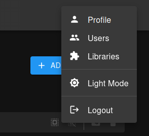
User menu (top-right corner) → Libraries
Once on the Libraries page:
- Click + Add and upload
forecast.zip - After the library is registered, go to the Diagnostic page and restart the Core service — the Forecast extension is activated during Core startup
- Core may take up to a minute to come back online; you may see temporary error messages in the UI during this process — this is normal
- Once Core is back, hard-reset your browser (
Ctrl+Shift+Ron Windows/Linux,Cmd+Shift+Ron Mac) to clear cached assets — without this the Forecast-related UI elements may not appear - The AI model is downloaded from HuggingFace on the first forecast request (~700 MB). This download can take several minutes — for short forecast horizons the prediction may be stale by the time it completes. Once the download finishes, re-run the forecast to get a fresh result. Subsequent startups use the local cache — no repeated downloads.
Enabling Forecast on a Chart
Open any chart’s Preferences panel and switch to the Forecast tab.
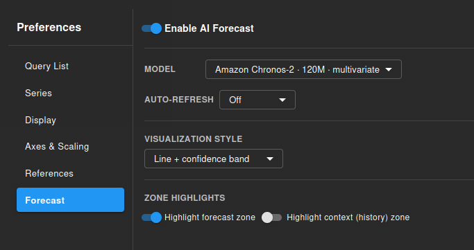
Chart Preferences → Forecast tab
| Setting | Description |
|---|---|
| Enable AI Forecast | Toggle to turn forecasting on/off for this chart |
| Model | Choose between Chronos-2 (120M, most accurate) and Chronos-2 Small (28M, faster) |
| Auto-refresh | Automatically re-run the forecast as the chart time window updates |
| Visualization Style | Line + confidence band or plain median line (default) |
| Zone Highlights | Shade the forecast zone and/or the historical context window on the chart |
Configuring a Forecast Run
Click the Forecast button on the chart toolbar to open the configuration dialog. This is where you assign roles to tags and define the forecast window.
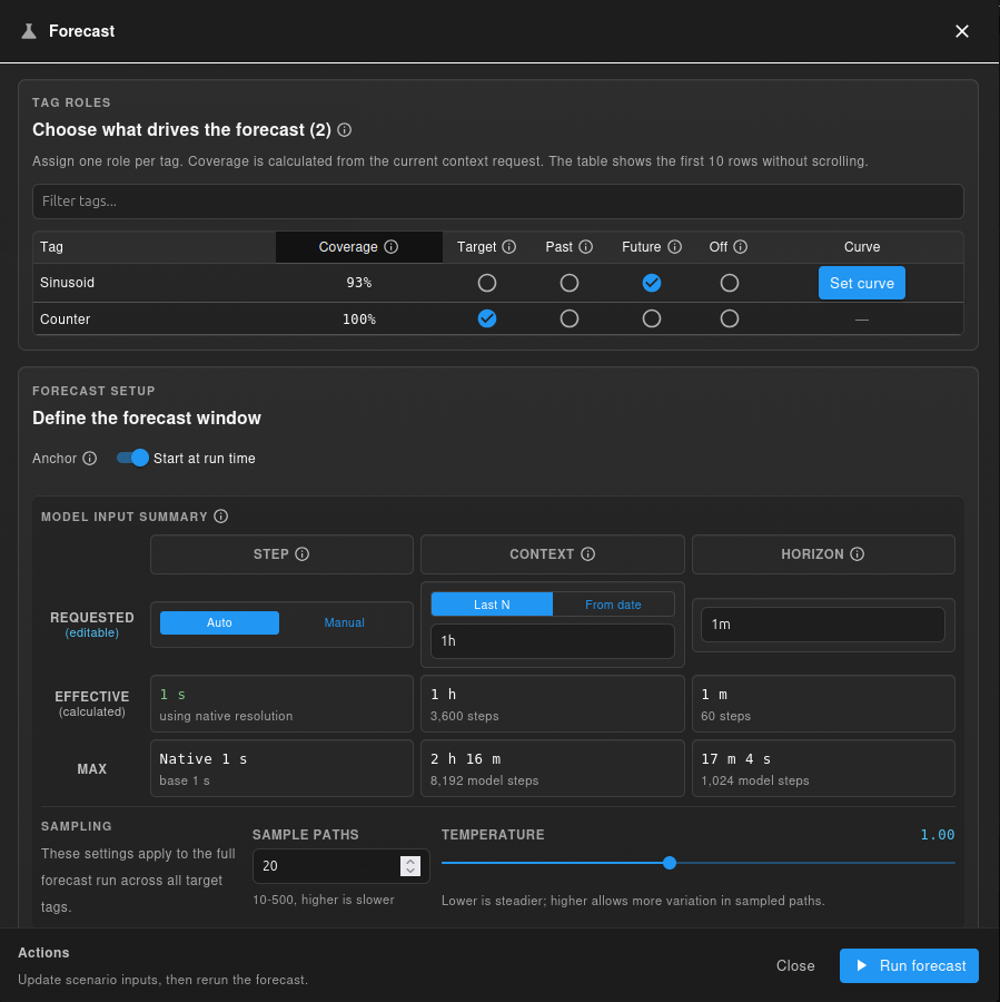
Forecast dialog — Tag Roles and window setup
Tag Roles
Each tag on the chart is assigned exactly one role:
| Role | Description |
|---|---|
| Target | The tag you want to forecast. The model predicts its future values. |
| Past | Provided as context to improve accuracy — the model sees its history but does not predict it. |
| Future | You supply a known or expected future curve for this tag (e.g. a setpoint). The model uses it as a covariate. |
| Off | Excluded from the forecast entirely. |
Multiple tags can be assigned Target — the model runs a joint multivariate forecast across all of them.
Forecast Window Settings
| Parameter | Description |
|---|---|
| Step | Time resolution of the forecast. Auto uses the tag’s native resolution. Set Manual to force a specific interval (useful to compress long horizons into 1,024 model steps). |
| Context | How much historical data to feed the model. Last N uses a duration (e.g. 1h). From date pins to an absolute start. |
| Horizon | How far ahead to predict (e.g. 1m = 1 minute). The effective number of steps is shown below. |
The MAX row shows hard limits based on the model: context is capped at 8,192 steps, horizon at 1,024 steps. If your step/context/horizon combination exceeds these, the step is auto-compressed and a warning appears.
Sampling
| Parameter | Description |
|---|---|
| Sample Paths | Number of random forecast trajectories the model generates (10–500). More paths = smoother confidence bands but slower inference. Default: 20. |
| Temperature | Controls spread of sampled paths (0–2). Lower = tighter/steadier band. Higher = more variation between paths. |
Future Curves
Tags assigned the Future role can have a custom curve drawn for them. Click Set curve next to the tag to open the curve editor.
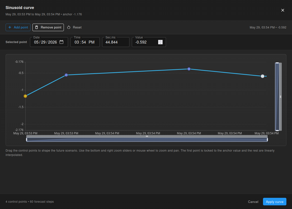
Future curve editor — drag control points to define the expected scenario
Drag the control points to shape the expected future value of the tag over the forecast horizon. The first point is locked to the anchor value (the last known value of the tag). Add or remove control points freely — the curve is interpolated between them. This lets you model “what-if” scenarios: what happens to temperature if we raise the setpoint like this?
Reading the Forecast on the Chart
Confidence Bands
The default visualization style shows a median line (dashed) surrounded by a confidence band — the shaded region represents the spread of all sampled paths between the 10th and 90th percentile.
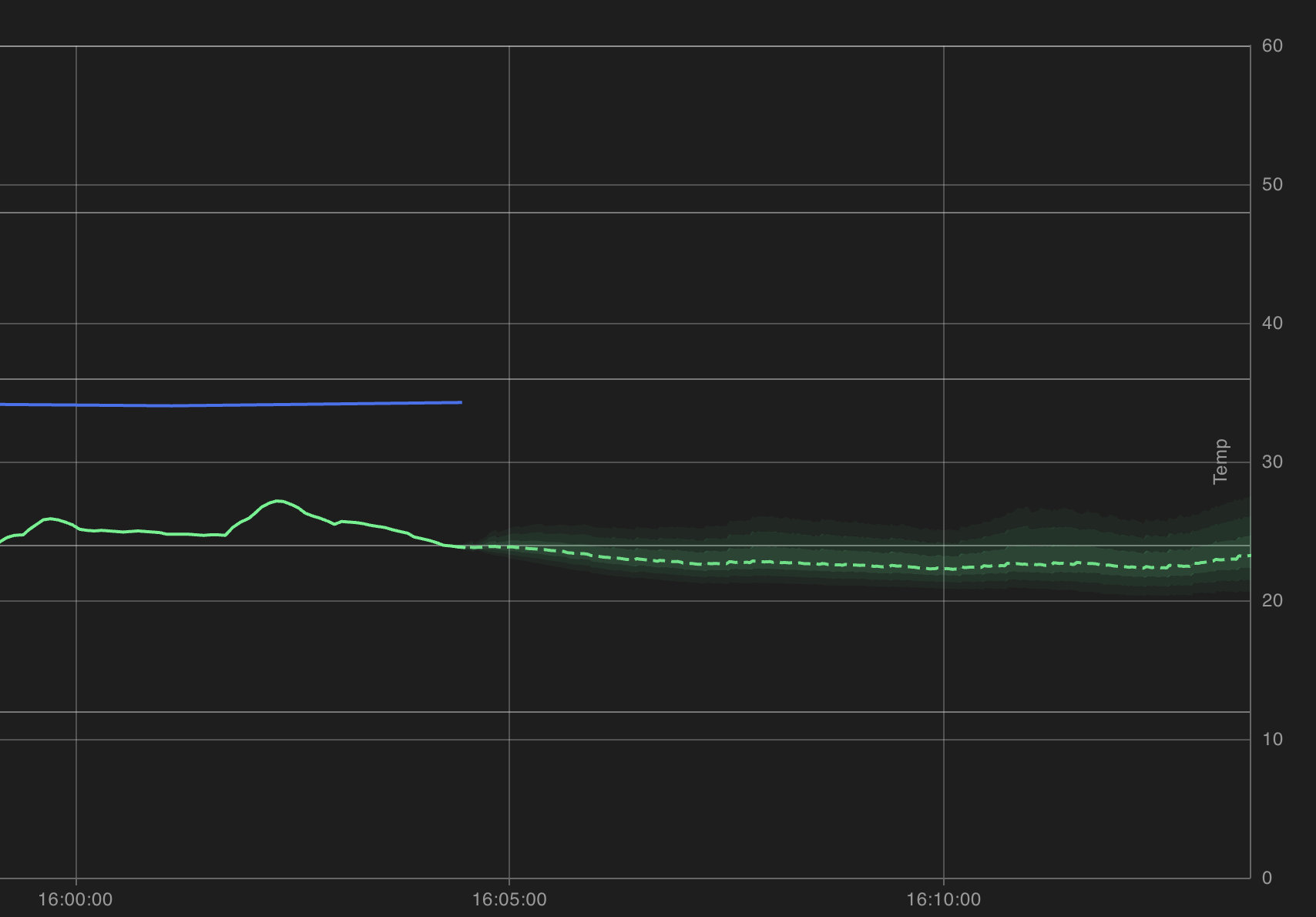
Solid line = historical data · dashed = median forecast · shaded band = confidence interval
A narrow band means the model is confident in its prediction. A wide band indicates more uncertainty — often seen when signals are noisy or the context window is short.
Legend and Series Names
Forecast series appear in the chart legend with an (F) suffix alongside the original tag name. Hover over the legend to highlight individual series.
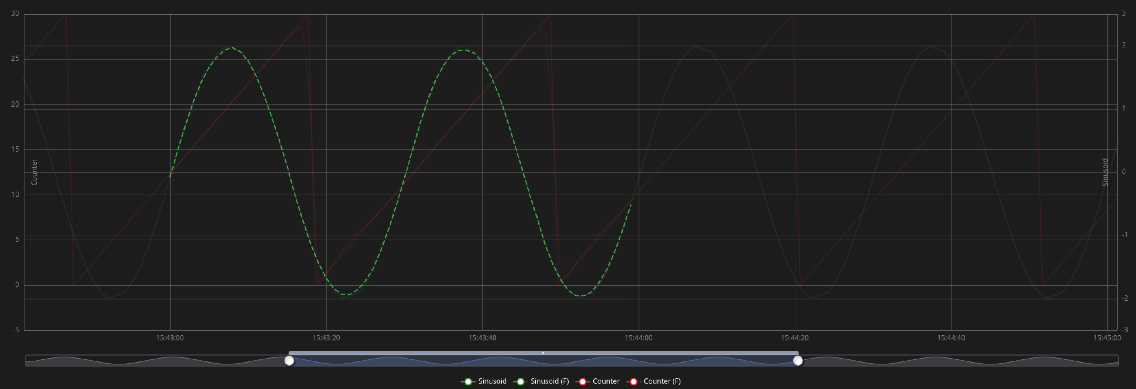
Legend showing original and forecast (F) series for each tag
Running on Historical Data
You can position the chart’s time window so the forecast runs against a past period. This is useful for validating model accuracy — compare the predicted trajectory against what actually happened.
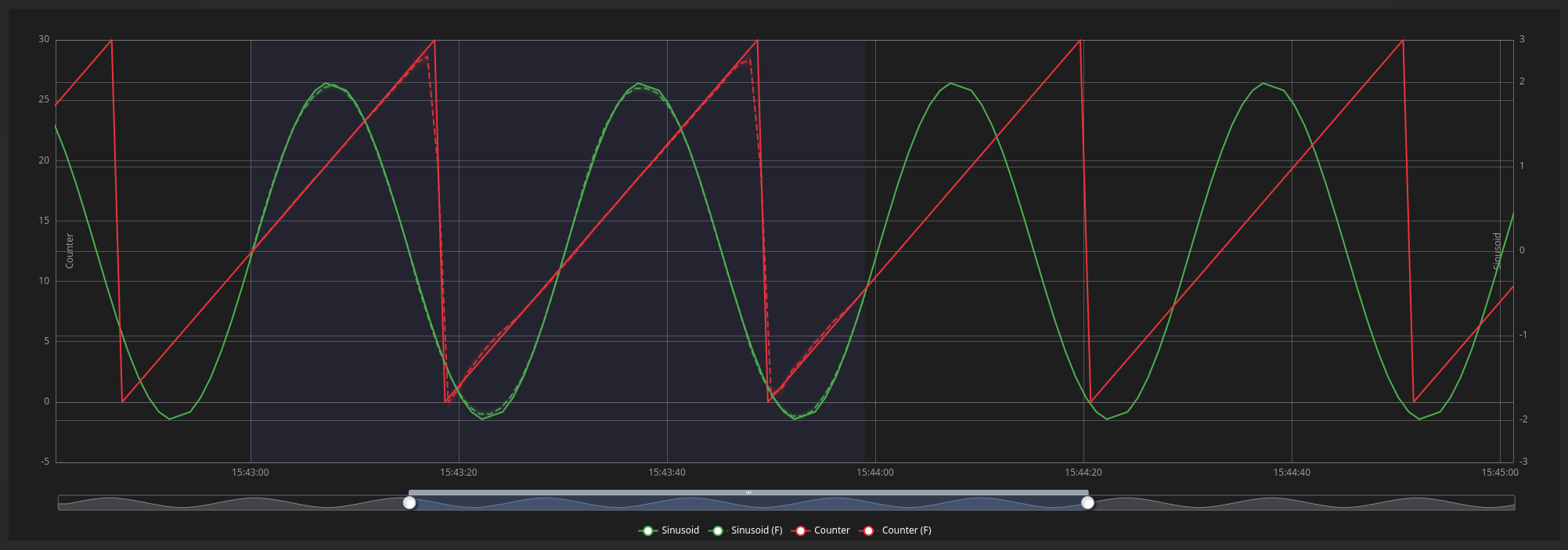
Forecast overlaid on historical data — highlighted zones show context (history) and forecast windows
The blue highlighted zones mark the context window (what the model saw) and the forecast window (what it predicted). Dashed lines are the forecast; solid lines are the actual recorded values. Both zone highlights can be toggled on or off individually via the Zone Highlights setting in the chart’s Forecast preferences.
Models
| Model | Parameters | Context limit | Horizon limit | Best for |
|---|---|---|---|---|
| Amazon Chronos-2 | 120M | 8,192 steps | 1,024 steps | Highest accuracy, multivariate |
| Chronos-2 Small | 28M | 8,192 steps | 1,024 steps | Faster inference, lower RAM |
Both models run on CPU — no GPU required. The model files are cached in var/hf-model-cache/ after the first download.
Troubleshooting
First forecast request times out The model is downloading in the background (~700 MB). Wait 2–5 minutes and click Run forecast again. Check progress with:
|
|
“Forecast service unavailable”
|
|
Confidence band is very wide Increase the context window, reduce temperature, or increase the number of sample paths.
Step auto-compressed warning Your horizon is too long for the native signal resolution. The model caps at 1,024 steps — the step is automatically increased to fit. Switch to Manual step to control this explicitly.
Model re-downloads on every restart
Check that ./var/hf-model-cache exists on the host and that Docker has write access to it.
Updating
When a new version of the Forecast extension is released, use an Update button on the extension card on the Libraries page. Click it, upload the new zip, then restart Core from the Diagnostic page and hard-reset your browser — the same steps as the initial installation.
Uninstalling
- Go to the Libraries page and remove the Forecast extension
- Restart Core from the Diagnostic page for the change to take effect
- Delete
var/hf-model-cache/manually to reclaim ~700 MB of disk space